Subsystem Modeling Theory
The following sections some of the engineering behind the models. Our main focus was to produce a model that predicts the instantaneous power required to run a transport capsule at the conditions specified in the original work. These power requirements are a function of the capsule air cycle and thermal conditions. The resultant power could then be combined with the estimated travel time to size the battery and coolant storage requirements. The following section provides a brief summary of the assumptions and modeling that went into each sub-system necessary to perform this analysis.
For the sake of conciseness, each section serves as a general summary. The reader is recommended to refer to the actual source code and included documentation for full implementation details. The current model omits economic, structural, safety, and infrastructure considerations; areas that become more prominent once the core engineering concept is deemed sufficiently feasible. These aspects are equally important to the overall design and they represent the next required step in producing a viable hyperloop design concept.
Compression System
- The compression system performs two functions on the hyperloop concept.
- Pressurizes some of the air, increasing its density, to provide a means of exceeding the Kantrowitz limit.
- Provides a source of high pressure air to the air bearing system.
Each of these functions requires that the compressors move a certain amount of air, which combine to define the total airflow for the whole sub-system. The system is comprised of an inlet, two compressors, two heat exchangers, a nozzle, and a duct to air bearings.
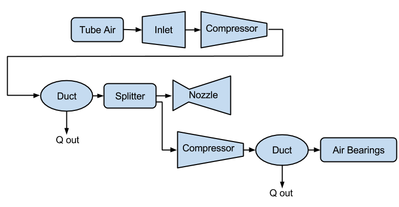
Schematic flow diagram of the compressor system
The compression systems is modeled as a 1-D cycle, representing components as a thermodynamic processes which are chained together. These models predict the instantaneous power consumption of the compression system.
Battery Pack
Tube Temperature
As each pod passes through the tube, it adds energy to the air in an amount equivalent to what was used to power the compressors. This added energy will cause a small temperature rise in the tube. Each pod causes an additional slight temperature rise as it passes, which could potentially heat the overall hyperloop system to excessive temperatures. In the original proposal, to combat this effect, it was proposed that water-to-air heat exchangers could be added to the compression system. These would use water stored in tanks in the pod to cool the air by converting it to steam. The steam could then be stored in an additional tank, and offloaded once the pod reached its destination. According to our initial calculations, using water for cooling is not an ideal design for two reasons:
1) The flow rate of water needed to remove the heat added by the compressors is very large, and storing the resulting steam would result in an unreasonably large pod (over 200 meters long).
2) The heat addition from each pod compressor cycle is fairly low relative to other heat transfer mechanisms, such as radiative solar heating of an uncovered steel tube. Even without an active on-board cooling solution, the tube temperatures may not reach excessive levels.
In the following two sections, we explain the analyses we used to draw the above conclusions.
Heat Exchanger Design
In spite of the results in the capsule cooling section, on-board cooling could possibly be used to partially fulfill cooling requirements. As a basic excercise a hypothetical baseline heat exchanger model was developed to investigate the weight and sizing requirements of an on-board water cooling system using the Logarithmic Mean Temperature Difference (LMTD) method. The exchanger was sized to remove all excess heat generated by the two compressors using a pedagogical shell and tube design. Based on the temperature restraints and exhaust flow rate determined by the cycle model, necessary water flow rates were calculated to ensure an energy balance. Given a predefined heat exchanger cross-section, fluid flow regimes and heat transfer coefficients were obtained. The combination of all of these elements provide a first-cut approximation of tank sizes, total heat exchanger volume, and pumping requirements.
Given:
-For simplicity, only a single heat exchanger is designed (to cool down the air coming off the first compressor stage)
-Sized as a classic shell and tube heat exchanger
-Input and output temperatures are known for each fluid
-Temperature change across the heat exchanger cannot be so large that Cp changes significantly
-Rigorously defined for double-pipe(or tubular) heat exchanger
With a chosen cross-sectional area of pipe and annulus, and known Q and mdot, the velocity of each fluid can be determined.
The hydraulic diameter (characterstic length) of a tube can also be calculated as,
Based on the geometry, kinematic viscosity \(\upsilon\), dynamic viscosity \(\mu\), thermal conductivity k, and velocity of the fluids the following non-dimension values can be calculated
Reynolds Number: (inertial forces/ viscous forces) \(Re = \frac{V D_{h}} {\upsilon}\)
Prandtl Number: (viscous diffusion rate/ thermal diffusion rate) \(Pr = \frac{C_{p} \mu} {k}\)
Based on the flow regimes determined above, the Nusselt Number.. can be calculated. The Dittus-Boelter equation is used in this case,
Nusselt Number: (convecive heat transfer / conductive heat transfer) \(Nu = 0.023*(Re^{4/5})*(Pr^{n})\) where n = 0.4 if the fluid is heated, n = 0.3 if the fluid is cooled.
Subsequently the convective heat transfer coefficient of each fluid can be determined, \(h = \frac{Nu*k} {D_{\varepsilon}}\)
All of these terms can then be used to calculate the overall heat transfer coefficient of the system,
This combined with the LMTD = \(\Delta {T}_{LMTD} = \frac{\Delta {T}_{2}-\Delta {T}_{1}}{ln(\frac{\Delta {T}_{2}}{\Delta {T}_{1}})}\) where \(\Delta {T}_{1} = T_{hot,in} - T_{cold,out}\) and \(\Delta {T}_{2} = T_{hot,out} - T_{cold,in}\)
allows the length to be determined for a single pass heat exchanger.
Further calculations for the multipass heat exchanger can be found in the source code.
References:
Cengal, Y., Turner, R., & Cimbala, J. (2008). Fundamentals of thermal-fluid sciences. (3rd ed.). McGraw-Hill Companies.
Turns, S. (2006). Thermal-fluid sciences: An integrated approach. Cambridge University Press.
Equilibrium Tube Temperature
A high-level assessment of the overall steady-state heat transfer between the 300 mile hyperloop tube and the ambient atmosphere was also investigated. The outer diameter of the pipe was chosen as the control surface boundary. Heat added from the capsule exhaust air and solar flux were considered the primary drivers for heat absorption into the tube. Heat released from the tube was modeled by means of ambient natural convection, and radiation out from the stainless-steel surface. The thermal interaction between the rarified internal air and tube was not modeled and assumed to reach steady-state in a reasonable period of time. These calculations served to approximate the necessary cooling requirements of the on-board heat exchanger given a certain steady-state heat limit within the tube.
The heat being added by the pods can be determined from the cycle analysis, or based purely on inlet total temperatures with isentropic flow relations.
Where PR is the compressor pressure ratio, MN is the mach number, \(\gamma\) is the specific heat ratio, and \({\eta}_{adiabatic}\) is the adiabatic efficiency.
With the air flow rate known, the heat flow rate per capsule is obtained,
The peak heating rate from the pods scales linearly.
The solar heat flow per unit area can be approximated, given the solar reflectance index (SRI) of stainless steel, non-normal incidence factor of the cylinder and solar insolation (SIF).
Multiplying this by the viewing area of the tube (assuming no shade and constant sun)
Tube cooling can be attributed to two general mechanisms, radiation and natural convection. Radiation power per unit area can be approximated to
where \(\epsilon\) is the emissivity factor and \(\sigma\) is the Stefan-Boltzmann constant.
Multiplying by the surface area of the tube, the total heating rate can be found,
Assuming the worst case scenario of no cross wind, convection is primarily driven by temperature gradients. The non-dimensional relation between buoyancy and viscousity driven flows is parameterized using the following imperical constants.
if 150 K < \(T_{amb}\) < 400 K:
if 400 K < \(T_{amb}\) < 2100 K:
The Grashof Number can then be approximated,
The non-dimensional Rayleigh number can then be calculated to estimate buoyancy effects, leading to the Nusselt number.
From this point the total heat transfer from natural convection can be obtained,
The steady state tube temperature can be found by varying the tube temperature until the rate of heat being released from the tube matches the rate of heat being absorbed by the tube. Using the values provided in the source code, a steady state temperature of 120 F was reached.
References:
https://mdao.grc.nasa.gov/publications/Berton-Thesis.pdf
3rd Ed. of Introduction to Heat Transfer by Incropera and DeWitt, equations (9.33) and (9.34) on page 465 <http://www.egr.msu.edu/~somerton/Nusselt/ii/ii_a/ii_a_3/ii_a_3_a.html>